Perform RNA-seq data analysis via using Rsubread and limma

Here we illustrate how to use two Bioconductor packages - Rsubread and limma - to perform a complete RNA-seq analysis, including Subread read mapping, featureCounts read summarization, voom normalization and limma differential expresssion analysis.

Case study

Data and software. The RNA-seq data used in this case study include four libraries: A_1, A_2, B_1 and B_2. A_1 and A_2 are both Universal Human Reference RNA (UHRR) samples but they underwent separate sample preparation. B_1 and B_2 are both Human Brain Reference RNA (HBRR) samples and they also underwent separate sample preparation. Note that these libraries only included reads originating from human chromosome 1 (according to Subread aligner). These read data were generated by the SEQC Consortium. The data used in this case study, including read data and reference sequence of human chromosome 1 (GRCh37/hg19), were put into a data package which can be downloaded from here (283MB).

After downloading the data package, uncompress it (do not uncompress the .gz files included in the data package) and save it to your current working directory. You need to have R installed on your computer to run this case study. You also need to have the following three Bioconductor R packages installed within your R: Rsubread, limma and edgeR. The version of Rsubread package should be 1.12.1 or later. You should run R version 3.0.2 or later.

If the required Bioconductor libraries were not installed in your R, you can issue the following commands under your R prompt to install them:

source("http://bioconductor.org/biocLite.R")
biocLite(pkgs = c("Rsubread","limma","edgeR"))

Preamble. Load libraries, read in names of FASTQ files and create a design matrix.

library(Rsubread)
library(limma)
library(edgeR)
options(digits=2)
targets <- readTargets()
celltype <- factor(targets$CellType)
design <- model.matrix(~celltype)
targets

  CellType  InputFile OutputFile
1        A A_1.txt.gz    A_1.bam
2        A A_2.txt.gz    A_2.bam
3        B B_1.txt.gz    B_1.bam
4        B B_2.txt.gz    B_2.bam

Index building. Build an index for human chromosome 1. This typically takes ~3 minutes. Index files with basename 'chr1' will be generated in your current working directory.

buildindex(basename="chr1",reference="hg19_chr1.fa")

Alignment. Perform read alignment for all four libraries and report uniquely mapped reads only. This typically takes ~5 minutes. The generated SAM files, which include the mapping results, will be saved in your current working directory.

align(index="chr1",readfile1=targets$InputFile,input_format="gzFASTQ",output_format="BAM",
output_file=targets$OutputFile,unique=TRUE,indels=5)

Read summarization. Summarize mapped reads to RefSeq genes. This will just take a few seconds. Note that the featureCounts function has built-in annotation for Refseq genes. featureCounts returns an R 'List' object, which includes raw read count for each gene in each library and also annotation information for genes such as gene identifiers and gene lengths.

fc <- featureCounts(files=targets$OutputFile,annot.inbuilt="hg19")
x <- DGEList(counts=fc$counts, genes=fc$annotation[,c("GeneID","Length")])

If you need RPKM values for genes, you can use the following command to generate them:

x_rpkm <- rpkm(x,x$genes$Length)

Filtering. Only keep in the analysis those genes which had >10 reads per million mapped reads in at least two libraries.

isexpr <- rowSums(cpm(x) > 10) >= 2
x <- x[isexpr,]

Normalization. Perform voom normalization:

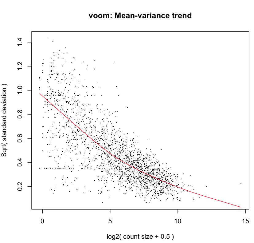
y <- voom(x,design,plot=TRUE)

The figure below shows the mean-variance relationship estimated by voom for the data.

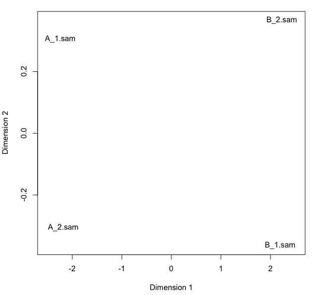
Sample clustering. The following multi-dimensional scaling plot shows that sample A libraries are clearly separated from sample B libraries.

plotMDS(y,xlim=c(-2.5,2.5))

Linear model fitting and differential expression analysis. Fit linear models to genes and assess differential expression using the eBayes moderated t statistic. Here we list top 10 differentially expressed genes between B vs A.

fit <- eBayes(lmFit(y,design))
topTable(fit,coef=2)

             GeneID Length logFC AveExpr   t P.Value adj.P.Val  B
100131754 100131754   1019   1.6      16 113 3.5e-28   6.3e-25 54
2023           2023   1812  -2.7      13 -91 2.2e-26   1.9e-23 51
2752           2752   4950   2.4      13  82 1.5e-25   9.1e-23 49
22883         22883   5192   2.3      12  64 1.8e-23   7.9e-21 44
6135           6135    609  -2.2      12 -62 3.1e-23   9.5e-21 44
6202           6202    705  -2.4      12 -62 3.2e-23   9.5e-21 44
4904           4904   1546  -3.0      11 -60 5.5e-23   1.4e-20 43
23154         23154   3705   3.7      11  55 2.9e-22   6.6e-20 41
8682           8682   2469   2.6      12  49 2.2e-21   4.3e-19 39
6125           6125   1031  -2.0      12 -48 3.1e-21   5.6e-19 39